uncertainty
overview
I added a measurement uncertainty engine to C47 on my DM42n. Enter the variables of a formula along with their standard uncertainties, and the calculator returns the result together with the uncertainty of that result, plus a budget showing which input is responsible for the error.
This is compliant with ISO/IEC Guide 98-3, the standard for stating measurement uncertainty. This is something you’d normally need a spreadsheet for, and rarely find in a basic calculator.
I got my inspiration here from DB48X, another firmware for the same hardware, which has an uncertain number type that propagates a standard deviation through operations. It lacks the rest of the ISO/IEC 98-3 stuff like sensitivity coefficients, a ranked budget, an expanded uncertainty with its coverage factor, effective degrees of freedom.
Oh, and I tried to make this run on the DM42 also, which is a capacity feat.
space
The DM42 has 704 KB of internal flash for the program. The firmware ships in numbered packages, which are different subsets of the features chosen to fit:
| package | flash used | free | engine |
|---|---|---|---|
| 1 | 721,808 / 720,896 | over by 912 | out |
| 2 | 720,680 / 720,896 | 216 | out |
| 3 | 719,528 / 720,896 | 1,368 | out |
| 4 | 699,040 / 720,896 | 21,856 | in |
Package 1 does not fit, and did not before I touched it: upstream is 784 bytes over on that package today. So three of the four have no room and the feature is compiled out of them.
The source keeps a calibrated table of what each option costs. Mine is 6,448 bytes of flash, measured by building package 4 twice with the option on and off.
step
The C47 uses a fifteen point stencil, exact for polynomials to degree fourteen, and then takes its step as h = x × 10⁻¹⁶. A central difference trades truncation error against rounding error and the balance sits near ε^(1/(p+1)); function values come back at 34 digits, so the optimum for that stencil is around 10⁻², not 10⁻¹⁶. At 10⁻¹⁶ the result is rounding noise and all fourteen orders are thrown away.
The firmware’s own checked-in test expectation for the first derivative of x³ at 5, which is 75:
74.99999999999999999893939393939394
20 digits out of 34. The second derivative gets 7.5, since dividing by h² amplifies the same noise.
So I did not reuse it. A two point central difference at h = max(|x|,1) × 10⁻¹¹ measures 22.6 digits using two evaluations instead of fifteen. Nearly three decades better for an eighth of the work. The sophistication was in the wrong place since the step decides whether the stencil matters at all.
Reading it also turned up four defects, the worst being that f’ and f“ returned a silently wrong answer for any program taking its input as a named variable. Fixed upstream now.
use
The UNCT menu structure looks as follows:
| U.EDIT | the input table, one row per variable: u(x) and degrees of freedom |
| U.CORR | correlations, if the inputs are not independent |
| U.P | level of confidence, 95 or 0.95, both work |
| U.CALC | y in Y, u_c(y) in X |
| U.EXP | k in Y, U in X |
| U.BUDG | the ranked budget |
| U.Y | which variable is the measurand, for a formula written with = |
A run is short. Pick the formula with EQN, then:
U.EDIT      fill in u for each variable
99 U.P      99 % confidence
U.CALC      50.000838 mm, u_c = 32 nm
U.BUDG      lS 25 nm, dtheta 16.68, d 9.7, dalpha 2.9
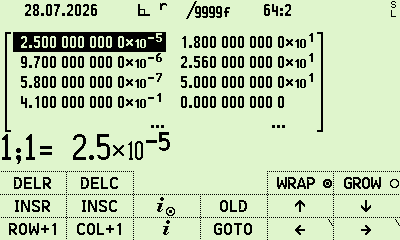
U.EDIT. One row per variable, u(x) in the first column and degrees of freedom in the second. Four of the six rows fit on screen.
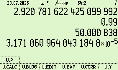
U.CALC on the GUM’s end-gauge example. 50.000838 mm in Y, 3.171×10⁻⁵ mm in X, which is 31.71 nm.
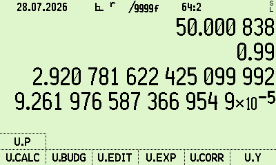
U.EXP at 99 %. k = 2.9208, U = 9.262×10⁻⁵ mm, the GUM’s 93 nm.
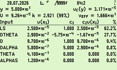
The budget. Six inputs ranked by what they contribute, LS at 62.2 % down to alphaS at nothing.
The combined number tells you how wrong you are; the budget tells you which measurement to go improve. Here it is LS, the calibration of the reference gauge, and no amount of care with the thermometer would help.
tests
The GUM contains its own worked examples in Annex H, with published answers. That is an unusually good acceptance test, because it was written by the people who defined the method.
The engine reproduces H.1, the calibration of an end gauge, giving 50.000838 mm with a combined uncertainty of 32 nm. It reproduces H.2, simultaneous resistance and reactance, which is the correlated example and exercises the covariance terms. It reproduces H.3, a thermometer calibration, both with and without the correlation between the fitted intercept and slope.
The GUM notes that including second order terms raises H.1’s uncertainty from 32 nm to 34 nm. This engine is first order by construction, so 32 nm is its correct answer, and getting 34 would mean the sensitivities were wrong. Encoding the number the approximation should produce, rather than the most precise number in the document, is the difference between a test that checks the method and a test that checks nothing.
cost
| flash | 6,448 bytes |
| static memory | 40 bytes |
| arena, on first use | about 2.2 KB |
| evaluations per budget | 2 per variable, plus one, except an = equation which is 2 per variable |
home | about | github | mastodon | rss

epoch
1789092085